3D animation of realtime data

3D animation of Satellite data

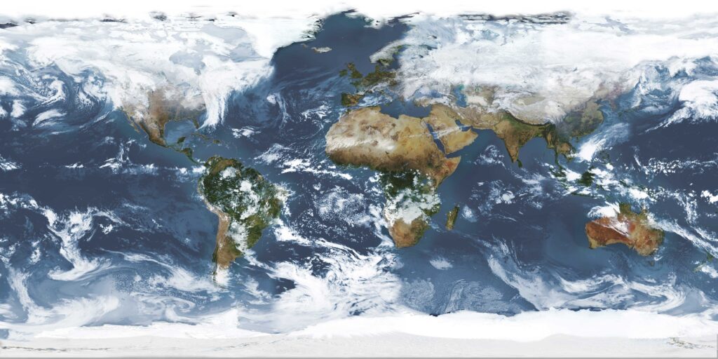
With the data I have been receiving from GOES 16-17 and Himawari 8 (via relay from GOES 17) I wanted to bump up the way I could visualize the imagery. So, using my data and adding downloaded data from Elecktro LN2, GK2A, I am able to compose a global composite through the use of the Sanchez tool. Using Sanchez’s built-in tools I take a series of images, from the same general timeframe. In these experiments, I used data I have from December 25, 2020 at roughly 14:00 UTC. I then combine all 5 satellites using Sanchez’ reprojection option and stitching option to make one flat equirectangular image of the earth:

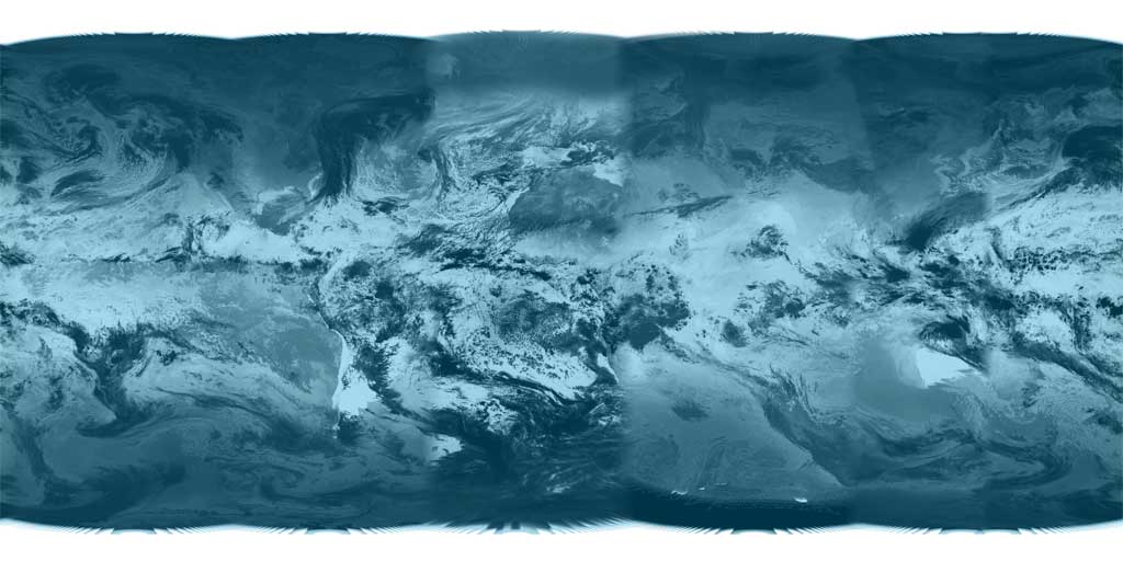
I also generate two additional files, a cloud layer file from the same data, this is done with no underlay.

Transparent cloud layer. Note you can see some of the areas where the satellite imagery is stitched. This will disappear on the rendered 3D imagery as I use just a slight transparency.

Once that is done, I typically resize the images down from the original size (too make it a bit faster in loading on the server.

Then the tricky part comes in. I am not going to go into a ton of detail on this as there are so mnay tutorials on this on the internet. I have used a combination of NASA World Winds software and a combination of three.js software, (A JavaScript-based library) and WebGL. Both when used are not for the faint of heart, It took me a manyf days to start rendering these 3D images.

The equirectangular views generated above are used to create my virtual planet earth. Each layer is placed as earth surface, earth cloud and earth cloud transparent. Each of these gives the visual perspective to look like a 3D object.

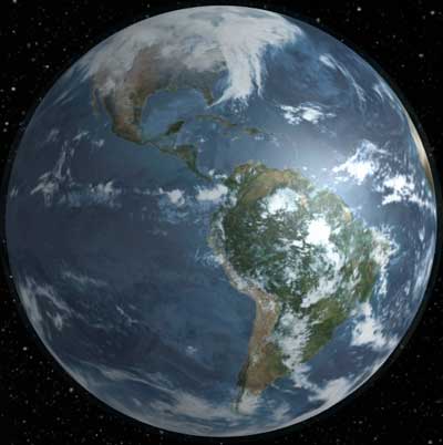
Layered 3D earth Using real satellite data.

Once those layers are all good, then the script with all the options I have chosen and set, build a virtual universe in which my little Class M planet will fit into. Bump maps are generated so that the sphere that the overlay is placed on can also show elevations, such as mountains or valleys, and a specular layer map is also used so that sunlight can glint off of water, just as lakes, streams, rivers, and oceans.

Here are a couple of examples showing the final results: You can control the view by clicking and moving your mouse around, and using your mouse wheel to zoom in and out.

Full Rendering of Earth with composited satellite imagery and a toolbar to control different settings. Uses the data from October 26,2022 (GOES 16-18 and Himawari 8, GK2A, Electro-L No. 2, and EWS-G1). This version uses a tiled star map and some fancy graphics to create a near photo-realistic universe. Cloud layer is turned off, try enabling it in the options to see the IR cloud imagery.

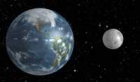
3D rendering of Planet Earth using data from October 26,2022 (GOES 16-18 and Himawari 8, GK2A, Electro-L No. 2, and EWS-G1

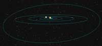
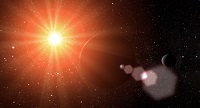
3D rendering of the solar system, with earth using the same data from October 26,2022 (GOES 16-178 and Himawari 8, GK2A, Electro-L No. 2, and EWS-G1 You can use the increase or decrease buttons to speed up or slow down the orbits. (My solar system still has Pluto as a planet!) The planets are layered with reprojected imagery from NASA JPL and http://planetpixelemporium.com/planets.html

Next steps: Automate the the stitching of imagery, reprojection using near realtime data, perhaps once per hour. Then use that imagery in combination with dark side imagery to create a near real time globe with options to scroll through dates and time.