Post Processing of received imagery.

So, for a little over two years now, I have been receiving, directly, GOES 16,17, and Himawari 8, along with various APT satellites like Meteor M2 and NOAA 15,18, and 19. I have stored about 3.8 Terrabytes of data from these sats, and, if you’ve been following along on my website, I a constantly trying to improve, modify, adapt, tweak and stretch what’s possible in the realms of post-processing the imagery. I have added MODIS and VIIRS Fire data to some, enhanced the false-color imagery, created new CLUTS to improve the gradients in specific bands, overlaid data from one sat onto another. And now I have taken the combined geostationary imagery I receive (or get from fellow amateur sat hunters) and created a new method of displaying this global imagery.

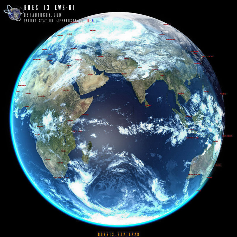
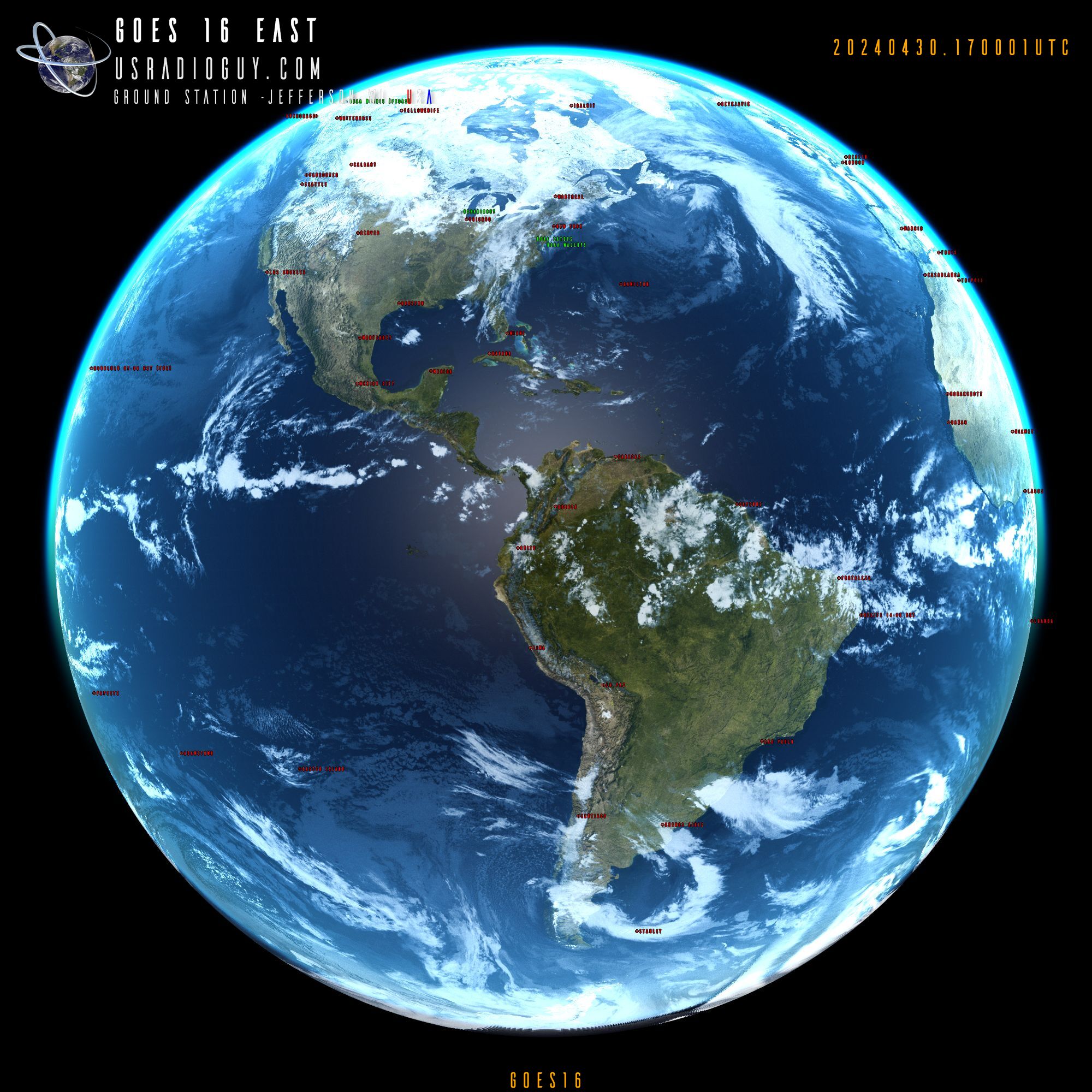
I have added to my website imagery that I receive and process using various pieces of software, all run from a single (though lengthy batch script) This imagery is compiled live (or as close to live as permissible) from 6 geostationary satellites, GOES 13, 16, 17, Himawari 8, GK2A, and Elektro L2. The imagery is created and uploaded to this site by my station twice daily. This is done, because, at any one time half the globe is in darkness. I have chosen to upload the imagery every day at 0900 UTC and 1800 UTC. (This helps conserve bandwidth and storage)

Global Composite Imagery from 6 Geo Stationary Satellites can be found by clicking here.

Adding Specular Lighting and Rayleigh Scattering to imagery.

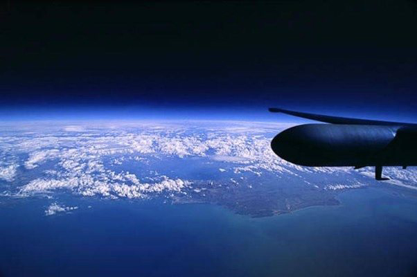
First off, what is Rayleigh Scattering?? You might have wondered why the sky is usually blue, yet red at sunset. The optical phenomenon which is (mostly) responsible for that is called Rayleigh scattering. When looking at imagery of the earth from space, especially from low earth orbit, one notices the atmosphere tinged in blue as the light passes through it to the observer’s eye. Since GEO sats are about 23,000 miles away, and the visible atmosphere is so thin, it becomes invisible to the spacecraft. I have found a method to replace that in full disk imagery from global GEO sats.

Additionally, I have added specular lighting to the earth imagery to represent the sunlight ‘glinting’ off of water (lakes and oceans).

Blue Sky ~Rayleigh Scattering

The interaction between light and matter is extremely complex, and there is no easy way to fully describe it. Modeling atmospheric scattering is, in fact, exceptionally difficult. Part of the problem comes from the fact that the atmosphere is not a homogeneous medium. Both its density and composition change significantly as a function of the altitude, making it virtually impossible to come up with a “perfect” model.

From a logical point of view, it makes sense that the strength of the scattering is proportional to the atmospheric density. More molecules per square meter mean more chances for photons to be scattered. The challenge is that the composition of the atmosphere is very complex, consisting of several layers with different pressures, densities, and temperatures. Luckily enough, most of the Rayleigh scattering happens in the first 60Km of the atmosphere. Within the troposphere, the temperature decreases linearly and the pressure decreases exponentially.

The blue color of the sky is caused by the scattering of sunlight off the molecules of the atmosphere. This scattering, called Rayleigh scattering, is more effective at short wavelengths (the blue end of the visible spectrum). Therefore the light scattered down to the earth at a large angle with respect to the direction of the sun’s light is predominantly in the blue end of the spectrum.

Note that the blue of the sky is more saturated when you look further from the sun. The almost white scattering near the sun can be attributed to Mie scattering, which is not very wavelength-dependent.

The water droplets that make up the cloud are much larger than the molecules of the air and the scattering from them is almost independent of wavelength in the visible range.

I have used a combination of software tools to achieve this phenomenon.

My basic workflow to achieve this:

1. Download from my local satellite recievers:
   1. GOES 16 Band 13
   2. GOES 17 Band 13
   3. Himawari 8 IR Imagery
2. Download from remote satellite servers:
   1. GK2A IR Imagery
   2. GOES 13 (EWS-G1) IR imagery
   3. Electro L2
3. Compile and stitch the imagery into a global composite using Sanchez to stitch the global composite.
4. Using Xplanet software:
   1. Create Rayleigh scattering lookup tables. Tables are calculated for fixed phase angles (the observer – point – sun angle). For lines of sight intersecting the disk, the tables are a 2D array of scattering intensities tabulated as a function of incidence (the zenith angle of the sun seen from the point of interest) and emission (the zenith angle of the observer seen from the point of interest).
   2. Specify Both Rayleigh Lighting and Specular Lighting in the config files for Xplanet.
   3. Using a subroutine in the batch file, I automatically generate all the differnet config files that xplanet needs to generate the imagery based on the files generated by Sanchez.
   4. Run Xplanet with the selected config to generate multiple planet views from each of the satellites longitude (ie GOES 16, -75.2° or GOES 13, 65°)
   5. If desired download the latest TLE’s for the selected satellites to place some satellite orbits on the map (in this case I used a few L.E.O. weather sats
   6. If desired select and use the Yale Bright Star Catalog to display, and name Stars.
   7. Generate a Full Global equirectangular image.